New Simulator

In order to solve this problem, it was necessary to write a new simulator to replace SPICE. This had a couple of big advantages. Firstly, it replaced the need for the tedious modification of the generator program, running the program to produce the SPICE file, transferring this file to SPICE, running SPICE, then transferring the SPICE output file to the decoder program before eventually examining the output. Secondly, because the simulator only had to deal with resistive fuse networks, it could be optimised and simplified for that application, making it many times faster. However, there was insufficient time to implement a completely accurate model of the operation of the resistive fuse circuit. Instead, it uses the ideal resistive fuse characteristic. The simulation results in Chapter 4 show that the actual operation of the circuits is close enough to ideal that it is reasonable to analyse the results of the simulator as though they came from a real circuit.

The simulator was written in C++. It has separate class definitions for Resistive Grid and Resistive Fuse Grid, so its operation can be easily switched between the two types of network, as well as the modified networks that were designed. The simulator used idealised models for the resistive fuse circuit, with perfectly linear behaviour in the conducting region and zero current in the cutoff region. The algorithm the simulator uses is based on Kirchoff's voltage and current laws. The simulator starts by approximating the output voltages as being the same as the input voltages. It then solves for the currents along each interconnection between output pixels. It then uses these currents to find new output voltages, and so on until the biggest change in output voltage between interactions is below some threshold. For these simulations, this threshold was 0.1mV, much higher than SPICE uses, but still satisfactory for the purposes of this work.

Furthermore, to improve convergence in a circuit in which small changes can produce dramatic effects, such as a whole chain of resistive fuses switching in a cascade, the solution was approached in a far more gentle fashion. At each iteration, a new solution for either voltage or current is deduced. Instead of replacing the old value with the new value, instead only a move of the 10% towards the new solution was made. This ensured that any dramatic cascades occur slowly, and that there was only a small amount of feedback at any point. The result of this was much improved convergence. Several different rates of convergence were tried, and it was found that 10% was the best figure to guarantee convergence. The source code for my simulator is on the floppy disk with this thesis.

Results from the simulator are shown in Figure 5.7. This is the same six pixel input pattern that was simulated by SPICE. As can be seen from this small simulation, the results are the same as a full SPICE simulation.

Figure 5.7: Simulation Results of Six Pixel Array.

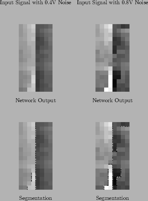
Figure 5.8 shows the results of simulations for various larger grids. The images were simple vertical edges with noise added to confuse the network. In these images, the input signal is of amplitude 0.5V, that is, the step between the light half and the dark half is 1V. The noise that was added was linearly distributed for each pixel between -0.4V and 0.4V for the first set of images, and -0.8V and 0.8V for the second set of images. They show that the resistive fuse has excellent performance at extracting the critical features from a noisy input signal. The main task of my honours project was to design a network that would improve on this performance.

Figure 5.8: Simulation of Larger Network.