Next: Conclusions Up: Other Network Topologies Previous: Hexagonal Grids Contents
The principles for connecting edge segments outlined in the previous section can be extended to apply to any arbitrary network topology.
The most general type of network topology would be the random grid, in which the pixels appear in totally random positions. Each pixel is then randomly connected with resistive fuses to some of its neighbours. Then, each resistive fuse is randomly connected to some of its neighbours by resistors. The question is, what weighting should be given to these links?
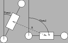
Consider the two edges shown in Figure 9.8. As for the two edges in the hexagonal grid, there is clearly going to be a relation between the differential voltage seen by the two resistive fuses. At most, they will be separated by a factor of the cosine of the difference between them. If we use this as a guide, then we can say that the strength of the resistance between any two resistive fuses in the grid should be
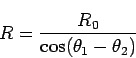
Where ![]() is the resistance of a parallel edge connection.
is the resistance of a parallel edge connection.
If the two edges were at right angles, this means that there would be no connection between them. If this principle was applied to a rectangular grid of pixels, then we would obtain the network that was discussed in Chapter 6. Thus, we can see that the principle provides an elegant link between the hexagonal resistive fuse network with two resistive grids added, and the rectangular resistive fuse network with four resistive grids added. Futhermore, this is starting to look much more like a biological neural system, in which the connections are not strictly defined on a uniform grid, but rather grow in a locally random manner, which produces a globally useful effect.
Matthew Exon 2004-05-23